
Nugget effect
There is a positive relationship between the occurrence of coarser gold (>100 µm) and nugget effect in a deposit. Nugget effect is minimal where the difference between original sample and adjacent sample have a value of zero or near zero value. The greater the variability between two adjacent samples, the greater the nugget effect and therefore, the uncertainty of the grade at that location increases (Clark, 2010). According to Dominy (2014), gold mineralization is susceptible to nugget effect, particularly those deposits containing coarser-grained gold.
Descriptive Statistics
The orebody modelling process, however simple or complex, is perceived to be a function of its geological characteristics (David, 1977). Geological and grade continuity can be established with appropriate drill spacing and sampling protocol but not with geostatistics. An example, a poorly drilled gold reef with extreme grades can only be estimated at a global scale (Dominy et al., 2001). Descriptive statistics are very effective tools when making decisions in regards to nugget effect, they include: histogram, boxplot, cumulative plot, probability plot and QQ plot, quantile, declustering and trend plots. These are early visual tools that assist with decision-making with regards to data distribution, whether the data is normal, lognormal, bimodally distributed or to simply compare two sets of data when there is reason to expect that they have similar distribution (Isaaks and Srivastava, 1989). Declustering the data is very important as there are drilling biases that can impact the resource estimation. Drilling is typically more concentrated in the high-grade areas in order to define the mineralization better (David, 1988). Using all the drillholes will over represent some areas and underrepresent in other areas (Figure 1).
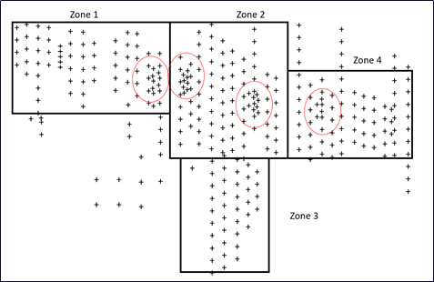
Figure 1: Regular and irregular (within red circle) drilling of uranium deposit in Saskatchewan. Modified from David, 1988.
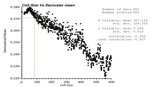
When debiasing the data, the best possible option is also to plot the declustered mean verses cell size and select the cell size that is appropriate for data distribution in X, Y and Z direction (figure 2).
Domaining and capping
Domaining and capping grade is important when dealing with nugget effect, one simple and effective tool is the use the coefficient variation (CV) range. If there are extreme values, they need to be treated. Coefficient variation is the standard deviation divided by the mean which measures variability in grade distribution:
CV= σ/m
If the CV value is >2.5, it indicates mix populations and warrants subsetting the data (Rossi and Deutsch, 2014). While other practitioners have indicated CV>1 point to the presence of erratic high value, which may influence the estimation (Isaaks and Srivastava, 1989). Extreme grade values can be viewed as an outlier in scattered, cumulative and probability plots, as they are represented by number of smalls but with extreme values, as shown in figure 3.
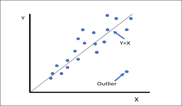
Figure 3: Scattered plot of paired of original and duplicate samples showing outlier. Modified from Babakhani, 2014.
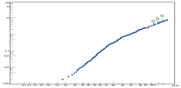
If a retested sample failed to confirm the original assay, it is considered an outlier and, in this case the sample should be documented and removed. Experts differ on how to treat extreme but confirming sample. Some prefer to cap the grade between 99.5% to 99.9% at the top of cumulative frequency distribution curve where the data disintegrates (Figure 4), while others follow the local custom of capping the grade at 1 oz/t or 28.35 g/t (Babakhani, 2014). The importance of the outlier is summarized in David (1988), particularly where the ore is custom milled by another company. If the company milling thinks the grade should be capped at certain grade, the company producing the ore is most probably cheated for resources. Cutting down outliers to a certain grade is the same logic as getting rid of the last cart on train carrying ore.
Variogram
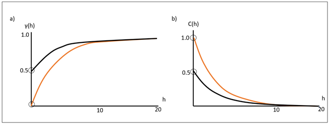
Variogram of γ(h) (figure 5, equation 1) measures the half average square difference between paired data value separated by some distance, and with increase lag distance, 2γ(h) and 3γ(h) are determined as represented by the brown circles in figure 5, this continues until there is no more sample autocorrelation and the variogram levels off.
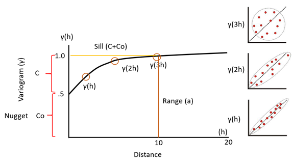
Equation 1 (Isaaks and Srivastava, 1989):
Sill: measures the total variance where the variogram levels off and the sill is often normalized to 1. Sill is defined as (C+ CO)
Range: A distance at which the semivariogram reaches the sill value. At this point, autocorrelation of samples is zero. Range is defined as (a)
Nugget: The nugget represents an extreme short-term variability between samples points (CO).
where ε% is nugget effect,
CO is nugget variance,
C is spatial variance,
and CO + C is total variance.
The ratio of nugget to sill is expressed at a percent:
low nugget effect, <25%
medium nugget effect 25–50%
high nugget effect, 50–75%; or
extreme nugget effect, >75%
Equation 1. Nugget (ε% ) as a function of variability in the grade.
Nugget effect can be zero at the origin of the variogram, or it can show vertical jump from the origin, caused by short term variability separated by extreme small distance, Figure 7. The best way to detect nugget value is to use omnidirectional variogram which has large directional tolerance; hence any separation distance becomes negligible, and what is important is the magnitude of the grade (h). The early use of omnidirectional is very important one because it combines multidirectional variogram into one. Omnidirectional serves as warning for erratic directional variogram. If the omnidirectional model doesn’t show a clear structure, directional variogram will also be messy. The lack of good structure in the omnivariogram may be indicative of one or more extreme values and it my warrant investigating and removing sample pairs. For a well behaved omnidirectional, one should move onto a directional variogram to figure out the maximum and minimum continuity and the anisotropic direction (Isaaks and Srivastava, 1989).
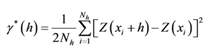
Those with values of more than 75% are likely to be the most challenging to evaluate. An example of pure nugget effect of (ε% ~ 100) is said to be totally random and difficult to estimate the grade of unsampled location, only classical geostatistics applies. (Dominy et al., 2001). Widely space drillholes cannot capture the short-term variability in the deposit. Semi-variogram calculation would give larger range for grade continuity in the major, minor and down dip axis, except where there is close space downhole data, which can then be used to define nugget effect. The short-term variability in the deposit can be decreased using large composites, but there is no correction possible for nugget effect produced from improper sampling, as this type of nugget effect is not random and not responsive to geostatistics. Sample error has a combining effect on the integrity of the data and hence, the sampler needs to follow proper procedures (Voortman, 1997; Neufeld, 2005). An example of two similar data is displayed in figure 6, one with no nugget effect and another with 50% of the sill and and where V represent the grade. Two separate variograms were calculated which resulted in a difference in calculated weight. Weight on data (a) appears to have a longer range between 0.057 to 0.318 while (b) shows shorter range between 0.125 to 0.178. The closer the kriging weight, the higher the estimate and kriging variance. The higher the nugget effect and the greater the smoothing of the estimate (Isaaks and Srivastava, 1989).
Figure 6: Ordinary kriging result showing a) kriging with no nugget effect where the range of weight assigned is between 0.06 to 0.32 b) kriging with pure nugget effect of 50% with weight range of 0.13 to 0.18. Modified from Isaaks and Srivastava, 1989).
Conditional Bias
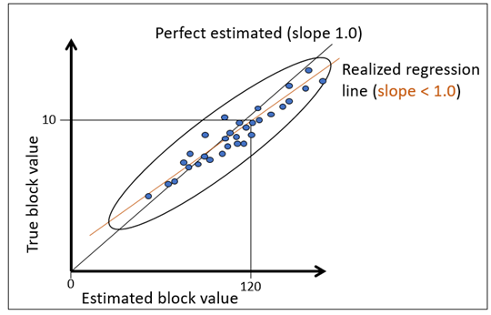
Once the grade is estimated, several methods exist to check if any biases may have been carried through. A block estimate can be checked against true value, if the true value is known.
True value is only possible if after estimation, the deposit is subsequently mined, and those grades are then plotted against the block grade. If the true value on the y (axis) and block value on the x (axis) matches well at 45% which has a slope of 1, the deposit is consider free of estimation error. If on the other hand it deviates from 45 degree, it points to error or conditional estimation bias, Figure 8. In most deposits where there is no historical mining grade, cross validation model is used. Cross validation would require variogram model, minimum and maximum sample, the output model is then plotted against the estimated grade.
The higher the nugget effect the greater the smoothing of the estimate. Therefore, to improve relationship between true and estimate value, It is possible to calculate regression slope of >0.95 as minimum slope for grade estimation efficiency by simply changing the block size, composite length and optimizing the number of samples used in the estimation (Krige, 1997; Voortman, 1997). Because nugget is isotropic, the effect of nugget can be lowered by increasing sample support.
Carrasco case study
The following figures 9 and 10, show two-real economic cases of what can happen when sampling procedures are not followed. The first case (figure 9) resulted an inflated nugget effect which undermined the kriging estimate. The precision of the estimate is very low and condition variance very high, causing a significant loss of Net Present Value (NPV) of $156 million AUD. (Carrasco, 2010). Figure 10 shows an improved case, where sampling protocol was followed. The estimation shows significant upscale with increased precision and the conditional variance had vanished. The new estimation reduced the NPV to $20 million AUD.
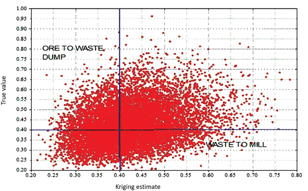
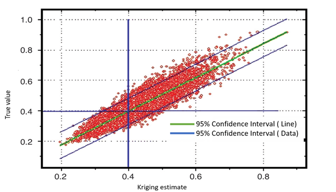
Figure 10: Improved sample protocol and sample support (Carrasco, 2010).
References
https://era.library.ualberta.ca/files/tx31qj23c/Babakhani_Mahshid_201404_MSc.pdf
Carrasco, P.C., 2010, Nugget effect, artificial or natural? The Journal of the South African Institute of Mining and Metallurgy, v. 110, p. 299-305.
Clark, I., 2010, Statistics or geostatistics? Sampling error or nugget effect? The Journal of the South African Institute of Mining and Metallurgy, v. 110, p. 307-312.
David, M., 1977, Geostatistical ore reserve estimation: Amsterdam, Elsevier Scientific Publishing Company, p. 345
David, M., 1988, Handbook of applied advanced geostatistical ore reserve estimation: Amsterdam, Elsevier Scientific Publishing Company, p. 1-39.
Dominy, S. C., and Annels, A. E., 2001, Evaluation of gold deposits—Part 1: review of mineral resource estimation methodology applied to fault- and fracture-related systems: Applied Earth Science, v. 110, p. 145-166.
Dominy, S. C., 2014, Predicting the unpredictable – evaluating high nugget effect gold deposits:
Mineral resources: Australasia institute of mining and metallurgy, 2nd edition, pp. 659-678.
Isaaks, E.H., and Srivastava, R.M., 1989, An Introduction to Applied Geostatistics: New York, Oxford University Press, 561p.
Krige, D.G., 1997, Block kriging and the fallacy of endeavouring to reduce or eliminate smoothing. 2nd Regional APCOM symposium, Moscow state mining university, p. 1-7
Rossi, M., and Deutsch, C., 2014, Mineral resource estimation: Statistical tools and concepts, Springer Dordrecht Heidelberg New York, pp. 11-26.
Simmonds, S-J., 2009, The nugget effects: In describing the variability of an ore deposit: Unpublished M.Sc. thesis, Grahamstown, South Africa, Rhodes University, 97p. Accessed on May 25, 2017;
Waberi, Hassan., 2017, Nugget effect: implication on resource estimation of gold deposits: Unpublished work
Voortman, L., 1997, How to optimize drillhole spacing and manage sampling errors: Australian Institute of Mining and Metallurgy, v. 6, p. 111-117.